Dimensionality reduction in machine learning and statistics is the process of reducing the number of random variables under consideration.
It is divided into 2 categories :
1) Feature Selection
2) Feature Extraction
Feature Selection : Reduce dimensionality by selecting subset of original variables. It finds interesting features from the original feature set.
Why Use Feature Selection? :
a) Simplifying or speeding up computations with only little loss in classification quality.
b) Reduce dimensionality of feature space and improve the efficiency, performance gain, and precision of the classifier.
c) Improve classification effectiveness, computational efficiency, and accuracy.
d) Remove non-informative and noisy features and reduce the feature space to a manageable size.
e) Keep computational requirements and dataset size small, especially for those text categorization algorithms that do not scale with the feature set size.
Some of Feature Selection Methods are :
1) TF and TF-IDF :
TF : In the case of the term frequency tf(t,d), the simplest choice is to use the raw frequency of a term in a document, i.e. the number of times that term t occurs in document d. If we denote the raw frequency of t by f(t,d), then the simple tf scheme is tf(t,d) = f(t,d).
IDF : The inverse document frequency is a measure of whether the term is common or rare across all documents. It is obtained by dividing the total number of documents by the number of documents containing the term, and then taking the logarithm of that quotient.
aking the idf(t,D) = log |D| / d Ɛ D : t Ɛ d
TF-IDF : tf–idf is the product of two statistics, term frequency and inverse document frequency. tfidf(t,d,D) = tf(t,d) * idf(t,D)
2) Mutual Information : Mutual information method assumes that the "term with higher category ratio is more effective for classification"
MI = log (A * N /((A+C)(A+B))
A : Number of document that contain term t and also belong to category c.
B : Number of documents that contain term t, but don't belong to category c.
C: Number of documents that don't contain term t, but belong to category c
D: Number of documents that don't contain term t and also don't belong to category c
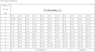
3) Chi Square : Chi square measures the lack of independence between a term t and the category, c
χ2 = N(AD-CB)2 / ((A+C)(B+D)(A+B)(C+D))
A,B,C,D as mentioned above and N is number of documents.
Through chi square value measure the p(significance value) from table as shown below :
Feature Extraction : It reduce dimensionality by (linear or non- linear) projection of D-dimensional vector onto d-dimensional vector (d < D).
The main linear technique for dimensionality reduction, principal component analysis, performs a linear mapping of the data to a lower dimensional space in such a way that the variance of the data in the low-dimensional representation is maximized.
principal component analysis(pca) Algorithm :
1) Create covariance matrix for features. covariance matrix (also known as dispersion matrix or variance–covariance matrix) is a matrix whose element in the i, j position is the covariance between the i th and j th elements of a random vector (that is, of a vector of random variables).
Covariance matrix shown beow :

It measure the relation b/w features.
Compute the "eigenvector" of covariance matrix ∑.
[u,s,v] = svd(covariance matrix ∑)
SVD : Singular Value Decomposition
SVD returns U matrix as shown below :

For calculating k dimensional z, we have to first take reduced dimension k column from U matrix.

Calculate Z from reduced U dimension as :

It can be write as :

It is divided into 2 categories :
1) Feature Selection
2) Feature Extraction
Feature Selection : Reduce dimensionality by selecting subset of original variables. It finds interesting features from the original feature set.
Why Use Feature Selection? :
a) Simplifying or speeding up computations with only little loss in classification quality.
b) Reduce dimensionality of feature space and improve the efficiency, performance gain, and precision of the classifier.
c) Improve classification effectiveness, computational efficiency, and accuracy.
d) Remove non-informative and noisy features and reduce the feature space to a manageable size.
e) Keep computational requirements and dataset size small, especially for those text categorization algorithms that do not scale with the feature set size.
Some of Feature Selection Methods are :
1) TF and TF-IDF :
TF : In the case of the term frequency tf(t,d), the simplest choice is to use the raw frequency of a term in a document, i.e. the number of times that term t occurs in document d. If we denote the raw frequency of t by f(t,d), then the simple tf scheme is tf(t,d) = f(t,d).
IDF : The inverse document frequency is a measure of whether the term is common or rare across all documents. It is obtained by dividing the total number of documents by the number of documents containing the term, and then taking the logarithm of that quotient.
aking the idf(t,D) = log |D| / d Ɛ D : t Ɛ d
TF-IDF : tf–idf is the product of two statistics, term frequency and inverse document frequency. tfidf(t,d,D) = tf(t,d) * idf(t,D)
2) Mutual Information : Mutual information method assumes that the "term with higher category ratio is more effective for classification"
MI = log (A * N /((A+C)(A+B))
A : Number of document that contain term t and also belong to category c.
B : Number of documents that contain term t, but don't belong to category c.
C: Number of documents that don't contain term t, but belong to category c
D: Number of documents that don't contain term t and also don't belong to category c
3) Chi Square : Chi square measures the lack of independence between a term t and the category, c
χ2 = N(AD-CB)2 / ((A+C)(B+D)(A+B)(C+D))
A,B,C,D as mentioned above and N is number of documents.
Through chi square value measure the p(significance value) from table as shown below :

Feature Extraction : It reduce dimensionality by (linear or non- linear) projection of D-dimensional vector onto d-dimensional vector (d < D).
The main linear technique for dimensionality reduction, principal component analysis, performs a linear mapping of the data to a lower dimensional space in such a way that the variance of the data in the low-dimensional representation is maximized.
principal component analysis(pca) Algorithm :
1) Create covariance matrix for features. covariance matrix (also known as dispersion matrix or variance–covariance matrix) is a matrix whose element in the i, j position is the covariance between the i th and j th elements of a random vector (that is, of a vector of random variables).
Covariance matrix shown beow :

It measure the relation b/w features.
Compute the "eigenvector" of covariance matrix ∑.
[u,s,v] = svd(covariance matrix ∑)
SVD : Singular Value Decomposition
SVD returns U matrix as shown below :
For calculating k dimensional z, we have to first take reduced dimension k column from U matrix.
Calculate Z from reduced U dimension as :
It can be write as :
No comments:
Post a Comment